Georeferencing in QGIS

QGIS is a great program and is a viable alternative to the old stalwart, ArcGIS. However, one aspect of ArcGIS that is vastly superior to QGIS is georeferencing maps. In ArcGIS, when you want to georeference a map, you simply load up the map, along with another pre-georeferenced image or map, click on the map you want to georeference, and then click on the place on the reference map that is equivalent. ArcGIS will then adjust the map you are georeferencing to account for the anchor point. This makes it a nice and easy workflow. If the map has known coordinates, you can right click and enter them.

QGIS offers a much more awkward way of georeferencing. The map you are georeferencing is placed in a separate window. Making an anchor point with an existing map can be awkward using the default settings, and as the version I am using (2.18.16), it is not possible to enter a geographic coordinate if you are using a projected coordinate system.

In addition to the above, there is not really a clear workflow tutorial on georeferencing in QGIS that I could find. I managed to make one up after some trial and error and finding information on places like Stack Overflow. I also had to tackle merging together scans of maps that were done in a piece-wise way. I am writing this so that I can look back to it in the future, but I also hope this proves useful to other people.

Getting started

The maps I want to georeference are some 1:500,000 Quaternary geology maps of Greenland. These maps were made in the 70s and 80s, and as of right now are not available online. The library at the Alfred Wegener Institute had them, but unfortunately did not have a scanner that was large enough to scan the entire map into one image. At first I thought it might be easiest to merge the scans using a photo stitching software (such as Hugin), but the results were less than satisfactory. The reason for this is because unlike photos, the maps have very little variance in colour, and the algorithms incorrectly warped and merged the images at the wrong places. It is much more effective to georeference the images individually in QGIS and merge them afterwards.

Keep in mind that the steps taken before will produce TIFF files by default, which may be quite large in terms of file size. Make sure you have a few GBs available (the final merged TIFF image in this example was more than 400 MB).

The first thing you have to do before you can georeference is to find out the projection the map is using. As you can see from, this information is not present on this map (always include this if you make a map!). You could always just use a geographic projection, as this has latitude and longitude values on it, but this will distort this map, which is not what you want. Luckily for me, one of the maps I had available did have information on the projection, and it was using a Universal Transverse Mercator (UTM) projection. This turned out to be the case for all of the maps I was georeferencing, but I had to make a guess as to the correct zone for each one. Don’t worry about cropping the scans where there is overlap and excess, this is something we will do later.

Reference maps

In order to georeference the map, we need something to reference to. Luckily, these maps have latitude and longitude graticules, and this is what I am using here as the reference. Initially I thought, “I can just enter the latitude and longitude values manually at each intersection”. This is indeed a plausible workflow if you are georeferencing to a geographic coordinate system, but this map is in a projected coordinate system. For whatever reason, the makers of the QGIS georeferencer did not include the functionality to convert geographical coordinates to projected coordinates. As a result, we need to create a grid that we can use as a reference. In the maps I have above, the graticule interval is 1° degree latitude and 0.5° longitude. QGIS has a handy way to construct a grid. First create a new project using a geographical coordinate system (the default is WGS84). From the pop-down menus:

Vector –> Research Tools –> Vector Grid

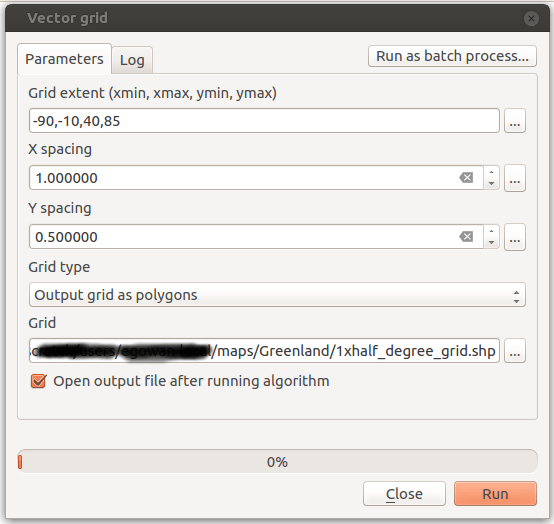
Here are the settings I used to produce the grid, keeping in mind that “x” is longitude and “y” is latitude. With the UTM projection we are using, try to ensure that your grid does not extent exactly to 90N, nor go too far east or west of the region of interest (in this case Greenland). If it does, when the grid is put into projected coordinates, it will bug out, and make QGIS work harder.

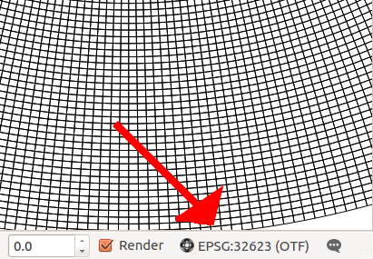
With that done, it is time to switch to the projected coordinate system. This can be done by hitting the button on the bottom right of QGIS. When the option box comes up, hit “Enable on the fly CRC transformation”, and search for the projected coordinate system, which in my case I guessed to be UTM 23N.

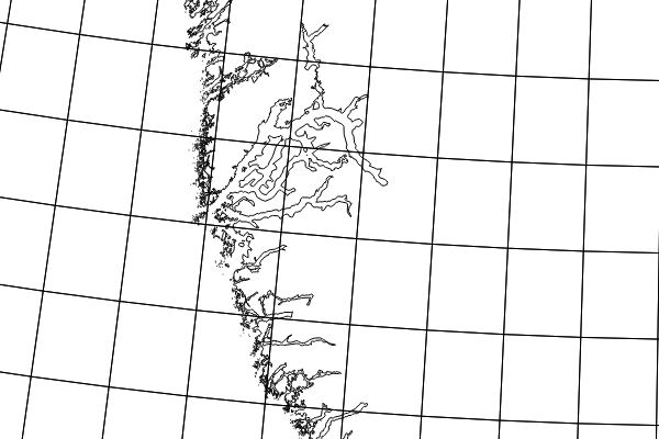
I am using this grid for the georeferencing, but since we are now using a projected coordinate system, the units are now in metres. Since it is hard to find the exact place where the map is from this, I also add shorelines the GIS. The GSHHG shoreline dataset is pretty convenient for this purpose.

Note that it is entirely possible to use the shorelines for georeferencing, but in this case I am not. There are a couple of reasons for this:

1. The shorelines in the GSHHG and the geological maps do not align in all areas. This is likely a result of errors in shoreline positioning on the geological maps, since they would have been created from surveys that predate satellite mapping. When digitizing, some shorelines matched well, in other areas it was off by up to 3 km. Using the shorelines will distort the map, and for my purposes it is not important to be that accurate.
2. The shorelines are features that are only along the edges of Greenland. Most of Greenland is a featureless ice sheet, and is surrounded by featureless ocean. Trying to use the shorelines for georeferencing will cause huge unwanted distortions in areas of the map that lack them.

If accuracy was important, I would probably use purely modern geographic sources for this information. Most of the information on these maps were likely created via air photo interpretation, so there likely are some errors anyways. Having strict accuracy is not crucial for my purposes.

Georeferencing the map

It is possible that the georeferencing plugin is not installed by default. To install it, go into the Install Plugins dialog and search for “Georeferencer GDAL”. After installing, make sure that you click on the box to make it active. Next open the georeferencer:

Raster –> Georeferencer –> Georeferencer

This will open the Georeferencer window. Before starting, go into the settings:

Settings –> Configure Georeferencer

The key option here is the “Show Georeferencer Window Docked” option. By default, the georeferencer is in a separate window. This gives it the extremely annoying property of minimizing the window every time you try to get a point from the reference map. This is especially annoying if you have a dual monitor setup, where you have the georeferencer in one window and the main QGIS window in another. By having the docked window, it will not do this, and it is entirely possible to drag it to another part of your screen. By doing this, you can visually see both the map you want to georeference, and the reference map at the same time. The only disadvantage is that there isn’t any “maximize” button, so you have to manually resize the window.

Go into the file menu and open up your scan (Open Raster). Before we start georeferencing, we need to make sure that the coordinate system is correct.

Settings –> Transformation Settings

In the above settings, make sure that the Target SRS is correct, which in our case is a UTM projection. You also have to set the Output Raster file name. You can also adjust the transformation type and resampling method. In my case, I have a relatively flat scan with few kinks, and I am using the same projection as the map, so a cubic polynomial is generally fine. If you were using a different projection from the map, or if the map is not scanned (i.e. a photograph), it is probably better to use a spline. The other option of note is the “Use 0 for transparency”. When I first started, I used this to cut out blank areas of the map, but my current workflow makes this unimportant, because we will be cropping the maps later using QGIS. Once you have referenced about 10 points, the georeferencing calculation will automatically update with every added point.

Now we can get started. Locate your scan with respect to the reference map. Next, zoom in on the feature on the map scan you want to match with reference. In my case, this is a gradicule interesection. Make sure to click on the “add point” button, and click the spot.

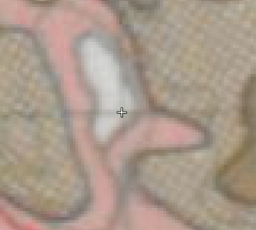
When you do this, a pop-up appears like this:

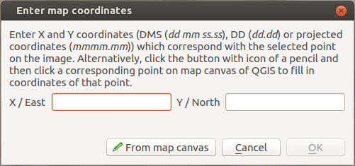
Despite what is implied in the wording, you cannot manually add the latitude/longitude values here, unless you are working in a geographical coordinate system. The program will not convert it to the projected coordinates automatically! Of course, many UTM maps also have the projected coordinates, so you could enter them here. Much more likely, it is easier to just grab the coordinates from the base map. Click on the “from map canvas” to do just that. There is no way that I could find to skip this pop up window and automatically get the coordinates from the map. So many clicks.

Next, you click on the equivalent spot on the reference map. In my case, it is the equivalent graticule intersection.

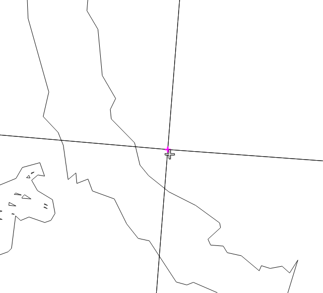
As you can see above, you don’t have to zoom and exactly click on the interesection, QGIS can snap to it. The pink crosshair indicates that you are snapped onto it. This is not on by default, so you have to do the following:

• On the Layers Panel, which shows the list of open layers, make sure that the grid layer is highlighted (click on it)
• From the drop down menus: Settings –> Snapping Options

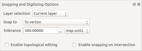
• Set the “Snap to” to “To vertex”, and use a generous Tolerance (here 500 m), and your cursor will automatically snap to the corner

After you click on the point on the reference map, it will extract the coordinates into the Extract map coordinates pop-up. Just hit ok, and the point will be added to the list.

Continue doing this until you have coverage over your whole map region. If your scan extends beyond the graticule intersections, the edges will be distorted. This is minimized if we are using the correct coordinate system for the map.

When you are happy with the amount of points, make sure to save them in case you are unsatisfied with the results and want to add more. The georeferencer does not automatically save the points when you close!

File –> Save GCP Points As

Next, hit the green arrow button, or go to the File menu and hit the options “Start Georeferencing”. With the options as above, it will open the georeferenced map into the main QGIS window. If the resulting map is highly distorted, and you are unable to add more points, you may need to change the Transformation type in the Transformation Settings. In the example below, the Polynomial3 transformation was bad (the reason for this is that the scan is just a vertically narrow chunk of the map), but changing it to “Helmert” gave a nice result. After doing this process with one of the scans, I got this:

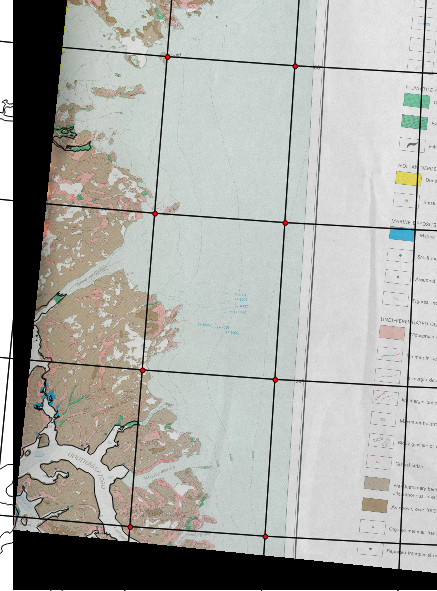
The georeferenced locations (red dots) match well with the georeferenced maps. Also the GSHHG shorelines (dark shoreline lines), match up well with what is on the scan. However, you can see the text and legend are at an angle. In the real map, it should be vertical. The projected coordinate system I used, UTM 23N, is incorrect! But this is a UTM projection, otherwise the map would be distorted and not fit so nicely. I switched to UTM 22N, and the map was in the correct orientation. However, this means all the georeferenced points are in the wrong spot, and you have to start over (or you can just leave the the coordinate system of the resulting raster as UTM 23N, then you don’t).

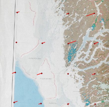
One thing to note, you know you have a georeferenced point wrong if there is a massive line going a point on the map you are georeferencing. You may want to delete it. The “delete point” option is kind of pain, since you have to click exactly on the point and they are tiny, but there really isn’t any other option except to try and find the point in the list, right click and delete. It can be hard to find which point is wrong, since a big line may be going from a point that is not wrong! Here is an example below:

Merging the map

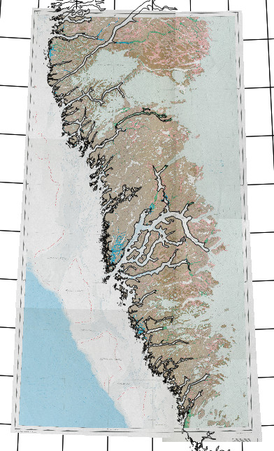
After doing the above process for each map, I get something like this:

All of the maps match to the graticules and shorelines fairly well. The next step is to merge everything together. There are varying levels of overlap between the map fragments, and is is ideal to crop out the edges of the scan, where the contact with the scanner was not great and caused the scan to be distorted. The middle of the scan should in theory be the least distorted, but it is best to visually compare and grab the area that conforms best to the base map. This is why I suggest cropping after the georeferencing step, rather than cutting it out prior to importing. This also allows us to create a clean transparency edges, which is not possible with the original jpeg files.

The first step you have to do is create a new polygon shapefile layer.

Layer –> Create New Shapefile Layer

Make sure the layer is in the same projection as your maps.

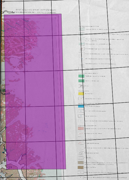
Toggle editing and draw a polygon around the the region you want to include in the final map, making sure to have some overlap with the adjacent maps to ensure there are no gaps.

To clip the map:

Raster –> Extraction –> Clipper

Make sure you:

• select the right input raster that you want to crop
• select an output file. If the file already exists and you want to overwrite it, you have to add the “-overwrite” flag to the gdalwarp command on the bottom!
• Select the No Data Value. By setting this, the selected colour will be rendered transparent in QGIS. By default it is 0 (black). If there is a lot of black colour on your map, it might be a good idea to change it to another colour.
• Select “mask layer”, and make sure to select the mask shapefile layer.

When you press ok, it will add the cropped raster to your map.

You need to repeat this process for each map. Make sure you delete the polygon you used to crop the previous map before you crop the next one. Unlike many tools in QGIS, the clipper does not recognize highlighted polygons, so you can’t just select one polygon from a shapefile with many polygons for the clipping.

After completing this, it is time to merge everything into a single raster.

Raster –> Miscellaneous –> Merge

 

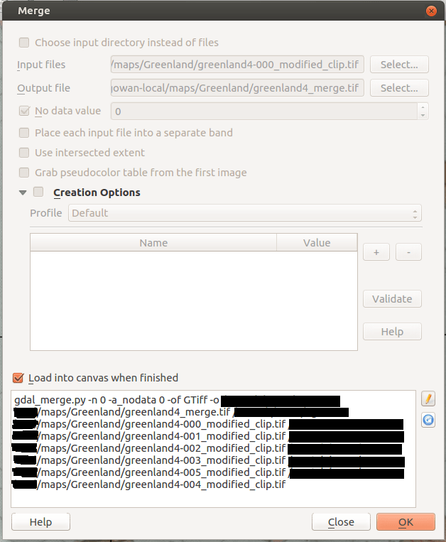
Here are the steps:

• Select all of the clipped raster files from the hard drive (no, it doesn’t let you select from loaded raster layers, which is annoying).
• Select an output raster name
• Check the “No data value” and make sure it is the same as what you were using before. If you don’t do this, all the overlapping clipped areas will be black.
• Edit the command line options so that the files are in the correct order. The rasters are merged sequentially, so in this case any area that is overlapping between “greenland4-000_modified_clip.tif” and the other rasters will be overwritten. In this particular case, I thought the overlapping region between 004 and 005 was better represented on 004.

After this we get the merged map:

From this zoomed out perspective, it looks pretty good, but let us zoom in where there are seams:

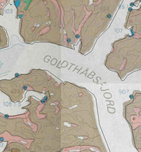
As we can see here, this place where three of the scans are overlapping has a bit of a discrepancy. In this location it is pretty good, maybe off by a couple of hundred meters, but in some places it is off by upwards of a kilometer. As noted above, there isn’t much you can do to improve this except by using a much more rigorous georeferencing process and using a spline, especially around the edges of the scan, which was not desirable in my case. For my purposes, this level of error is acceptable.

I hope this explanation is useful for other people. It is mostly just for me to reference if I ever have to do this again in the future!